With the inevitable development of technology, various businesses around the world have started to use cloud services more and more. First, let’s explain what cloud technology is and what it serves us for. Cloud technology, cloud security or as it is otherwise known as cloud computing includes a series of mechanisms that cooperate with each other to provide businesses and companies worldwide with a high level of security. Now the data, information and database of companies that were once stolen by other people are safe.
If we use cloud technology and cloud security, we will not have to worry about the unwanted flow of information. Great care must also be taken in choosing cloud services, who they offer in the market and which is the best option for us to choose. There are many companies in the world that would offer us cloud services for a fee, but we must carefully study which one benefits us the most.
Using these services today has many, many advantages. One of the biggest advantages is the reduction of time. Think about how much time we would save if all our data and information could be saved with just one click without having to save them manually one by one. Another advantage for the company would be the reduction of staff and, as a consequence, savings on workers’ salaries.
Think about it, if cloud technology was enough to store the company’s data and it would solve the problem with one click, would we need security workers? Consequently, no. What would this mean? This would mean not only reduction of staff but also saving of income. In a few words, cloud technology is trying to get closer to as many businesses in the world as possible by means of improvements and regular updates, meeting their needs. In conclusion, cloud technology is becoming a necessary and irreplaceable service* all over the world from which all businesses are being run every day and more.
One of the best services offered by cloud technology is the adaptation to different applications.
In this case we will talk about private clouds. Previously we talked about private clouds, how they help in the management of supermarkets, while this time we will talk about how cloud technology also helps restaurants.
As many of you already know, everywhere in the world restaurants are also being digitized. The best way to manage it is to install applications on servers.
The number of workers and managers varies from one restaurant to another. However, the staff cannot be called small, while there can be staff starting from 7 people in one shift. Well, in the metropolis, the restaurants are big and have a lot of staff. There are many managers, cooks, assistant cooks, waiters and assistant waiters. (Remember that restaurants also have other employees such as economists and cleaners, but this is not the case).
What is one of the most important in installing applications is the menu? Menu and rating of restaurants.
If you go to a restaurant, you will see a QR code on the menu, which allows you to read the menu with smartphones. And finally, after you have been served and consumed the meal, you can evaluate the service, the quality of the food and the prices. You, as a customer, are in control of the ranking and prestige of the restaurant.
In any case, we cannot leave without mentioning that all these achievements are possible thanks to applications, websites and cloud technology.
Data disposal and memory are key points in technological maintenance. The people who are in charge of the development of technology and applications are Developers.
When we enter the house and see the furniture and electrical appliances, we must think about how we can update or upgrade. Yes, these are the right words. Devices such as air conditioners, boilers, vacuum cleaners, washing machines, stoves and cleaning robots have managed to be controlled by phones. Of course, the relevant applications are not lacking.
How are household appliances connected to smartphones?
A very interesting question. Programmers and developers everywhere in the world think about objective things. They use technology and cloud services to configure smartphone programs with air conditioners, stoves, cars, robots, etc.
Thanks to cloud technology (in this case, private cloud), it is possible to control different home devices with suitable applications.
As you know, the most typical device is the air conditioner. Houses equipped with air conditioners of the latest technology have finally solved the problem of temperature adjustment.
Example: suppose you’re coming home from work and it’s scorching hot outside. In the car, you are in the fresh air of the air conditioner, only 25°C, while outside the temperature is 40°C. If you were to get out of the car and immediately enter the house at room temperature, then the first thing you would do would be to change your clothes. This is because you will sweat profusely within 3 minutes. Well, since you have a smartphone and a state-of-the-art air conditioner, you can control your air conditioner from the car and set it to the desired temperature through an application. Not bad, right?
Software engineers are computer scientists who utilize engineering concepts and linguistic expertise to construct software products, design computer games, and operate network control systems.
The number of software engineers is only increasing, with more and more of us depending on smart gadgets, with employment prospects expected to climb at 21 percent over the next nine years.
Types of Software Engineers
The field of software technology is large. Developers have many settings of technological skill, from computer building, network safety, and websites that target customers.
There are two main software engineers: software developers for apps and software developers for systems.
Applications Software Developers
Client-focused End-user interaction design software Develop iOS, Android, Windows, Linux, and other applications Analysis of prerequisites for conduct Regularly update the program and release
Systems Software Developers
Create user-facing operating systems and networks Responsible for software and hardware requirements Integration on one platform of diverse software products They often function as IT managers or architects of systems IT standards design and implementation Maintain information technology documentation and updates
How to Become a Software Engineer
Before, the only way to effectively begin a career as a software engineer was with a two- or four-year computer science degree. Furthermore, other graduate degrees in mathematics and other sciences have allowed people to go into software development. Such as IT, electronics, and civil engineering, or even community college training.
But a formal degree or some university curriculum is not the only way to build online. Bootcamp coding is an increasingly popular alternative for individuals who wish to switch to software technology rapidly.
Before choosing a program, consider what kind of career you are searching for and which language to study. Having offices in New York? See 10 free classes in NYC for more details.
You need to construct the portfolio and update your Software Engineer Resume after your course is complete.
Vector analysis, a mathematics subject that deals with both size and direction quantities. The magnitude of some physical and geometrical values, termed scalars, can be completely specified in appropriate measuring units.
More and more weight, the temperature in grams and time in seconds can indicated on some scale. In certain numerical scales, scales can graphically represented as points, such as a clock or thermometer. There are other quantities that need direction and magnitude definition, termed vectors. Examples of vectors are speed, strength, and displacement. A vector quantity can graphically represented by an arrow pointing to the vector quantity, denoted by a directed line segment, which is the length of the segment expressing the vector magnitude.
Vector algebra.
A vector prototype is a guided section of the line AB (see Figure 1). It might considered that a particle would displaced from its original point A into a new position B. Vectors have usually referenced using boldface characters to distinguish from scalars.
More, in Figure 1, the vector AB can represented by a length (or size) |a|. In many cases, the location of a vector’s starting point has irrelevant. Such that two vectors have considered equal provided their length and direction have the same.
The equality of 2 vectors a and b has indicated by the conventional symbolic notation a = b and helpful definitions are provided by the geometry of the fundamental algebraic operations of a vector. More, if the movement from A to B of the particles has represented by AB=a in Figure 1.
Further More, the portion has then moved to a location C in the case of BC=b, then it has appeared that the movement from A to C may be carried out with a single AC = c movement. So the writing of a +b = c is reasonable.
A, B Vector
This structure of sum, c, a, and b is equally similar to the parallelogram Act in which diagonal ACs of the parallelogram built on the AB and AD vectors as sides produce the resulting c. Because the position of the vector beginning B B = b is irrelevant, BC = AD has followed. Figure 1 demonstrates the AD + DC = AC for switching legislation
Holds the added vector. Also, the association law is straightforward to illustrate.
The parenthesis in (2) has legal and can thus removed without ambiguities.
When s is scalar, sa is a vector with a length of |s||a| and the direction of which is positive in a when s and negative in contrast to that of a when s. A and an are, thus, vectors of identical size but opposite directions. The above definitions and the widely known characteristics of scalar numbers (as seen in s and t) indicate that.
Since legislation (1), (2), and (3) have similar laws in normal algebra. It has quite proper for systems with a linear equation containing a vector to solved by familiar algebraic rules. It enables many synthetic geometry theorems, which require complex geometrical structures, to derived by solely algebraic techniques.
Products of vectors.
The vector reproduction leads to two types of products, the dot product, and the cross product. The dot or scale of two vectors a and b, written a·b, is a true number |a||b|cos (a,b), where (a,b) indicates an angle of a to b. Geometrically,
If a and B are in the right corner, a·b = 0, and if a b is not a zero vector, the vector is perpendicular to the disappearance of the dot product. When the square of a length has given a = b then cos (a,b) = 1, and a·a = |a|2. For the dot multiplication of vectors, associative, commutative, distributive, and fundamental algebra rules apply.
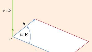
The vector of two vectors (a and b), abbreviated a stand b, is the cross- or vector product
where n is a unit length vector perpendicular to plane a and b and therefore a right-handed screw rotated from b to b moves towards n (see Figure 2). If a and b are parallel, then a = b is equal to 0. The size of the parallelogram with a and b as neighboring sides can equal the magnitude of paragraph b. Since the rotation between b and b is opposite,
This indicates that the product cross is not switchy, but the associative rule (sa) = B = s(a = b).
are valid for cross products.
Coordinate systems.
Given the lack of specific or accidental selections of reference frames established as physical relations and geometric configurations in the empirical laws of Physics, vector analysis is an appropriate research tool for the physical universe.
The introduction of a specific frame of reference or coordination system creates a correspondence of vectors and numbers that are the components of vectors in that frame and gives rise to certain operating rules for those numbers which follow the rules for the line segments.
If a particular set of three non-colinear vectors has picked, then every vector A may uniquely represented as a parallelepiped diagonal whose borders form part of A in the direction of the basis vectors. The axes of the famous Cartesian frame have guided by a set of three mutually orthogonal unit vectors (e.g. length vectors) 1 I j and k. (see Figure 3). The expression takes shape in this system.
where x, y, and z are the projections of A upon the coordinate axes. When two
vectors A1 and A2 have represented as the use of laws (3) yields for their
sum
Thus, in a Cartesian frame, the sum of A1 and A2 is the vector determined by (x1 + y1, x2 + y2, x3 + y3).
Also, the dot product can be written since
The use of the law (6) yields so that the cross product is the vector determined by the triple of numbers appearing as the coefficients of i, j, and k in
Data redundancy comes when the same piece of data has kept in two or more separate places and is a typical occurrence in many organizations. As more organizations have shifting away from walled data to using a single repository to hold information, they have discovering that their database has packed with inconsistent copies of the same entry. While it is difficult to reconcile – or even benefit from— redundant data inputs, it may help alleviate your enterprise’s long-term inconsistencies by learning, how to effectively eliminate and track data duplication.
How does data redundancy occur?
Data redundancy sometimes occurs by mistake, and others are deliberate. Accidental redundancy of information can emerge from a complicated, or inefficient coding method whereas deliberate redundancy has utilized to preserve the data and to maintain consistency — simply by utilizing the numerous occurrences and quality controls of data for disaster retrieval. If duplication is deliberate, a central area or data room must be available. This allows you to update all redundant data records if needed. If duplication has not intended, it can lead to a number of problems we will describe in the following.
Understanding database versus file-based
The database, the organized collection of structured data saved on a computer system or the cloud, provides data duplication. A distributor can have a database to track its stored items. If two errors occurred in the same product, data duplication occurs. The same distributor can store client files in the file system. When a consumer purchases more than once from the firm, its name might inputted several times. Redundant data has believed to be duplicate customer name records.
Whether in a database or in a file storage system duplication arises, it might be an issue. Data replication can, fortunately, assist avoid duplication by storing the same data in several locations. Companies may maintain consistency and obtain the information they need at all times through data replication.
A database is an organized data collection such that it is accessible, maintained, and updated simply. Computer databases normally include data or file aggregations, information on selling transactions, or customer interactions.
The digital information on a certain client in a relational DB has arranged into indexed rows, columns, and tables. So that relevant information may easily found through SQL or NoSQL queries. A graph DB , by contrast, employs nodes and edges to establish connections between information inputs and queries that need a unique semantic search vocabulary. SPARQL has the only semantic query language accepted by the World Wide Web Consortium (W3C).
Users often have the option of checking read/write access, specifying reporting, and analyzing use via the DB manager. Some databases offer ACID compliance to make sure that data are consistent and transactions complete (atomicity, consistency, insulation, and durability).
Types of database
Since their foundation in the 1960s databases has developed from hierarchical. Network databases to object-based databases in the 1980s, to SQL, NoSQL, and cloud databases. Bibliographic, full-text, numeric, and pictures can categorize according to the kind of material from one perspective. In computers, their organizational style sometimes classifies databases. The most common method, relational databases, distributed databases, cloud databases, graph databases, or NoSQL databases are all distinct types of databases.
Relational database
Invented at IBM by E.F. Codd in 1970, a relational database has a table DB in which data have defined to rearranged and retrieved for a variety of purposes. A number of tables containing data that fall into the designated category have formed related databases. Each tab has at least one data category in each column. For the categories set forth in the columns, each row includes some data instance.
Structured Query Language (SQL) is the default user interface for relational databases. Relational databases have easy to expand. Additional databases may added without requiring you to alter any apps. Once you have created the first DB .
Distributed database
A distributed database is a database that stores sections of the DB in a number of physical places and disperses and replicates the processing between several points in a system. Homogeneous or heterogeneous datasets might distributed. All physical sites within a single, distributed database system have equipped with the same underlying hardware and operate the same operating systems and applications. Each location may have various hardware, operating systems, or database software in the heterogeneous distributed database.
Cloud database
A cloud-based database is an optimized or constructed database on a hybrid cloud, public cloud, or private cloud for a virtualized environment. Cloud databases offer advantages. Such as the option to pay-per-use for storage capacity and bandwidth. Offer high availability and scalability on request. A cloud database also allows companies to enable business applications. With the deployment of software as a service.
NoSQL
For big collections of dispersed data, NoSQL databases are beneficial. For Big Data performance problems, NoSQL databases are efficient to resolve relation databases. They have best done when a company has to examine huge portions of unstructured information or data stored in the cloud over several virtual servers.
Object-oriented
Object-oriented programming languages frequently store things in relational databases, while object-oriented databases are suitable for such objects. An object-oriented database has organized around objects, not activities, and not logic. A multimedia record in a relational database might for example, instead of an alphanumeric value, be a defined data object.
Graph database
A NoSQL database type that employs graph theories to store, map, and query connections is a graph-oriented database or graphical database. Graph databases are fundamentally node and edge collections, where each node represents a whole and each edge constitutes a link between nodes. The popularity of graph databases for the analysis of linkages is rising. For instance, corporations might utilize a graph database to collect data about social media consumers.
SPARQL, a declarative language of programming and protocol for graph database analysis has commonly used by graph databases. SPARQL can do all the analytics that SQL can do and can used to analyze relations, semantical analyses, and analyses. This makes it helpful for analyses of both organized and non-structured data sources. SPARQL enables users to analyze information held in the relationships and Friend of a Friend (FOAF), PageRank, and Shortest route information in a relational database.
Advantages
1. Improved data sharing: The DBMS creates an environment in which end users have greater and better-managed access to more information. Such access allows end-users to swiftly adapt to environmental changes.
2. Improved data security: The more the dangers of data security violations, the more people access data. Corporations devote significant time, effort, and money to guarantee the correct use of business data. A DBMS offers a framework for improved privacy and security enforcement of data.
3. Better data integration: Enhanced access to well-managed data supports an integrated perspective and a sharper understanding of the company’s activities. How activities in one area of the business influence other segments are much simpler to discern.
4. Minimized data inconsistency: Incompatibility of the data occurs when multiple versions of the same data emerge at separate locations. For example, data discrepancy occurs when a company sales department has “Bill Brown” as its sales representative, and the staff department of the company stores “William G. Brown” as the same person, or the regional sales department has a price of $45.95 as the regional sales bureau of the company and the national sales department has the same price as $43.95. In a correctly constructed database, the chance of data incoherence is significantly minimized.
5. Improved data access: The DBMS enables fast replies to ad hoc requests. For the database, an inquiry is a specific request for data manipulation given to the DBMS, for instance for reading or updating the information. Just stated, a question is a matter, and an ad hoc question is a matter of the present. The DBMS returns a response to the application (called the query results set). End users, for instance.
Disadvantages
1. Increased costs: Database systems demand highly experienced individuals and complex software and technology. The costs of maintaining a database-hardware, system software, and staff can be significant. When database systems are installed, training, licensing, and regulatory compliance expenses are sometimes ignored.
2. Management complexity: Database systems demand highly experienced individuals and complex software and technology. The costs of maintaining a database-hardware, system software, and staff can be significant. When database systems are installed, training, licensing, and regulatory compliance expenses are sometimes ignored.
3. Maintaining currency: You must maintain your system up to date to optimize the efficiency of your database system. Thus, you must often update and apply all components with the newest patches and security measures. Due to constantly advancing database technology, staff training expenses tend to be high. Dependency of the seller. Due to substantial investment in technology, organizations may be unwilling to shift providers of databases.
4. Frequent upgrade/replacement cycles: DBMS manufacturers often add new functions to improve their systems. Often these new features are grouped into new software upgrades. Some versions of these need modifications to the hardware. It costs not only money to upgrade, but also money for the training of users and administrators in using and managing the new features.
A linked list is a linear data structure that does not store the members at adjacent memory locations. In the related Links, the components are connected using points. A linked list of nodes comprises basic words, where each node has a data field and a reference(link) to the following node in the link.
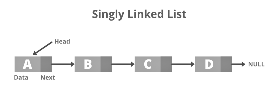
Singly Linked List
This is the simplest type of related Link in which every node holds certain information and a reference to the following node of the same data type. The node carries a reference to the following node, meaning that the node stores in the following node address. Only one direction can a single related Links travel data. The picture for the same is below.
Structure of Singly Linked List
// Node of a doubly linked list static class Node { int data;
// Pointer to next node in LL Node next; };
//this code is contributed by ali
Creation and Traversal of Singly Linked List:
// Java program to illustrate // creation and traversal of // Singly Linked List class GFG{
// Structure of Node static class Node { int data; Node next; };
// Function to print the content of // linked list starting from the // given node static void printList(Node n) { // Iterate till n reaches null while (n != null) { // Print the data System.out.print(n.data + ” “); n = n.next; } }
// Driver Code public static void main(String[] args) { Node head = null; Node second = null; Node third = null;
// Allocate 3 nodes in // the heap head = new Node(); second = new Node(); third = new Node();
// Assign data in first // node head.data = 1;
// Link first node with // second head.next = second;
// Assign data to second // node second.data = 2; second.next = third;
// Assign data to third // node third.data = 3; third.next = null;
printList(head); } }
// This code is contributed by Ali
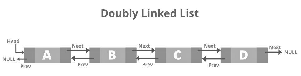
Doubly Linked List
A double-related Links or a two-way listed link is a more complicated form of a listed link that has a sequential indicator for the next node and the previous one. Hence it comprises three pieces of data. An indicator for the next node. An indicator for the previous one. This would allow us also to go back through the list. The picture below is identical.
Structure of Doubly Related Links
// Doubly linked list // node static class Node { int data;
// Pointer to next node in DLL
Node next;

// Pointer to the previous node in DLL
Node prev;
};
// This code is contributed by ali
Creation and Traversal of Doubly Related Links:
// Java program to illustrate // creation and traversal of // Doubly Linked List import java.util.*; class GFG{
// Doubly linked list // node static class Node { int data; Node next; Node prev; };
static Node head_ref;
// Function to push a new // element in the Doubly // Linked List static void push(int new_data) { // Allocate node Node new_node = new Node();
// Put in the data new_node.data = new_data;
// Make next of new node as // head and previous as null new_node.next = head_ref; new_node.prev = null;
// Change prev of head node to // the new node if (head_ref != null) head_ref.prev = new_node;
// Move the head to point to // the new node head_ref = new_node; }
// Function to traverse the // Doubly LL in the forward // & backward direction static void printList(Node node) { Node last = null;
System.out.print(“\nTraversal in forward” + ” direction \n”); while (node != null) { // Print the data System.out.print(” ” + node.data + ” “); last = node; node = node.next; }
System.out.print(“\nTraversal in reverse” + ” direction \n”);
while (last != null) { // Print the data System.out.print(” ” + last.data + ” “); last = last.prev; } }
// Driver Code public static void main(String[] args) { // Start with the empty list head_ref = null;
// Insert 6. // So linked list becomes // 6.null push(6);
// Insert 7 at the beginning. // So linked list becomes // 7.6.null push(7);
// Insert 1 at the beginning. // So linked list becomes // 1.7.6.null push(1);
System.out.print(“Created DLL is: “); printList(head_ref); } }
// This code is contributed by Ali
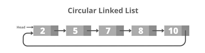
Circular Linked List
A circular related Links holds the pointer to the initial node of the list. While we go through a circular. We may begin at any node and go back. Forth through the list in any direction until we have reached the same node that we started. So there is no start and no end to a circular related Links. The picture below is identical.
Structure of Circular Related Links:
// Structure for a node static class Node { int data;
// Pointer to next node in CLL Node next; };
// This code is contributed by ali2110
Creation and Traversal of Circular Related Links:
// Java program to illustrate // creation and traversal of // Circular LL import java.util.*; class GFG{
// Structure for a // node static class Node { int data; Node next; };
// Function to insert a node // at the beginning of Circular // LL static Node push(Node head_ref, int data) { Node ptr1 = new Node(); Node temp = head_ref; ptr1.data = data; ptr1.next = head_ref;
// If linked list is not // null then set the next // of last node if (head_ref != null) { while (temp.next != head_ref) { temp = temp.next; } temp.next = ptr1; }
// For the first node else ptr1.next = ptr1;
head_ref = ptr1; return head_ref; }
// Function to print nodes in // the Circular Linked List static void printList(Node head) { Node temp = head; if (head != null) { do { // Print the data System.out.print(temp.data + ” “); temp = temp.next; } while (temp != head); } }
// Driver Code public static void main(String[] args) { // Initialize list as empty Node head = null;
// Created linked list will // be 11.2.56.12 head = push(head, 12); head = push(head, 56); head = push(head, 2); head = push(head, 11);
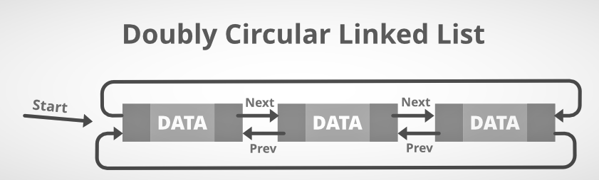
A dubious situation A circular related Link or a circular linked double-way list is a more complicated form of a connected list that contains both the next and the last nodes in the sequence. The difference between the two doubling lists is the same as between the one-bound list and the one-bound list. In the preceding field of the first node, the circulated double-related Links does not include null. The picture for the same is below.
Structure of Doubly Circular Related Links:
// Structure of a Node static class Node { int data;
// Pointer to next node in DCLL
Node next;

// Pointer to the previous node in DCLL
Node prev;
};
//this code is contributed by ali2110
Creation and Traversal of Doubly Circular Linked List:
// Java program to illustrate creation // & traversal of Doubly Circular LL import java.util.*;
class GFG{
// Structure of a Node static class Node { int data; Node next; Node prev; };
// Start with the empty list static Node start = null;
// Function to insert Node at // the beginning of the List static void insertBegin( int value) { // If the list is empty if (start == null) { Node new_node = new Node(); new_node.data = value; new_node.next = new_node.prev = new_node; start = new_node; return; }
// Pointer points to last Node
Node last = (start).prev;

Node new_node = new Node();

// Inserting the data
new_node.data = value;

// Update the previous and
// next of new node
new_node.next = start;
new_node.prev = last;

// Update next and previous
// pointers of start & last
last.next = (start).prev
    = new_node;

// Update start pointer
start = new_node;
}
// Function to traverse the circular // doubly linked list static void display() { Node temp = start;
System.out.printf("\nTraversal in"
    +" forward direction \n");
while (temp.next != start)
{
    System.out.printf("%d ", temp.data);
    temp = temp.next;
}
System.out.printf("%d ", temp.data);

System.out.printf("\nTraversal in "
    + "reverse direction \n");
Node last = start.prev;
temp = last;

while (temp.prev != last)
{

    // Print the data
    System.out.printf("%d ", temp.data);
    temp = temp.prev;
}
System.out.printf("%d ", temp.data);
}
// Driver Code public static void main(String[] args) {
// Insert 5
// So linked list becomes 5.null
insertBegin( 5);

// Insert 4 at the beginning
// So linked list becomes 4.5
insertBegin( 4);

// Insert 7 at the end
// So linked list becomes 7.4.5
insertBegin( 7);

System.out.printf("Created circular doubly"
    + " linked list is: ");
display();
} }
// This code is contributed by Ali
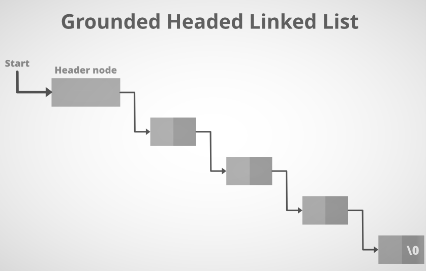
Header Linked List
A linked list header is a particular form of related Links containing a header node at the start of the list. START will thus not point at the initial node of the list in header-related Links, but START will include the header node address. Below is the picture of the related Links Grounded Header.
Structure of Header Linked List:
// Structure of the list static class link { int info;
// Pointer to the next node
link next;
};
// this code is contributed by Ali2110
Creation and Traversal of Header Linked List:
// Java program to illustrate creation // and traversal of Header Linked List
class GFG{ // Structure of the list static class link { int info; link next; };
// Empty List static link start = null;
// Function to create header of the // header linked list static link create_header_list(int data) {
// Create a new node
link new_node, node;
new_node = new link();
new_node.info = data;
new_node.next = null;

// If it is the first node
if (start == null) {

    // Initialize the start
    start = new link();
    start.next = new_node;
}
else {

    // Insert the node in the end
    node = start;
    while (node.next != null) {
        node = node.next;
    }
    node.next = new_node;
}
return start;
}
// Function to display the // header linked list static link display() { link node; node = start; node = node.next;
// Traverse until node is
// not null
while (node != null) {

    // Print the data
    System.out.printf("%d ", node.info);
    node = node.next;
}
System.out.printf("\n");

// Return the start pointer
return start;
}
// Driver Code public static void main(String[] args) { // Create the list create_header_list(11); create_header_list(12); create_header_list(13);
// Print the list
System.out.printf("List After inserting"
    + " 3 elements:\n");
display();
create_header_list(14);
create_header_list(15);

// Print the list
System.out.printf("List After inserting"
    + " 2 more elements:\n");
display();
A Logic structure is essentially a block of programming that examines variables and determines a direction in which to move depending on specified parameters. The phrase flow control specifies the direction the program goes (which way program control “flows”) (which way program control “flows”). Hence it is the primary decision-making process in computers; It is a forecast.
Types of Logic Structure
Algorithms and their equivalent computer programs have more easily understood if they mainly use self-contained modules and three types of logic, or flow of control, called.
Sequence logic, or Sequential flow
Selection logic, or conditional flow
Iteration logic, or repetitive flow
These three types of logic have discussed below, and in each case, we show the equivalent flowchart.
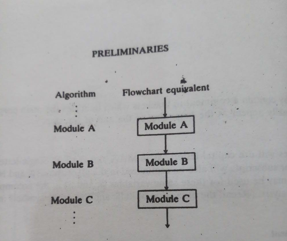
Sequence Logic (Sequential flow)
The rationale of the sequence had explored before. The modules have performed in the obvious sequence unless otherwise instructed. The order in which the modules have drawn may shown openly, via numbered stages, or implicitly. (See pictures 2-3). This basic flow pattern usually has followed by most processing, even complicated situations.
Selection Logic (Conditional flow)
The selection logic uses a variety of conditions that allow one of a number of possible modules to selected. The structures implementing this logic have referred to as conditional structures or structures. To clear, the end of such a structure has often indicated by the declaration.
[End of If Structure]
These conditions are described in three types, which have individually explored.
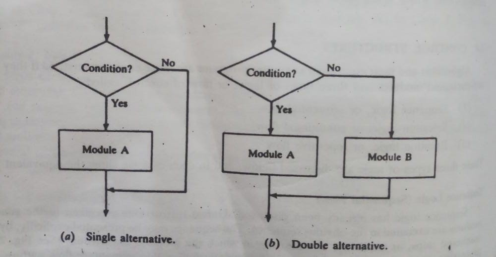
Single alternative. This structure has the form
If condition, then:
[Module A]
[End of if structure]
If the condition is present, then Module A has run, which could consist of a further statement; otherwise, Module A has skipped and the transfer of control to the next phase of the algorithm is controlled.
2. Double alternative. This structure has the form
If condition, then:
[Module A]
else:
[Module B]
[End of if structure]
If a condition is present, Module A will run, as shown in the flowchart; module B otherwise will executed.
If condition(1), then:
[Module A1]
else if condition(2), then:
[Module A2]
else if condition(M), then:
[Module AM]
else:
[Module B]
End of if structure]
The structural logic enables the execution of just one of the modules. Specifically, it executes either the module after the first condition or the module following the last sentence Else. More than three choices will hardly occur in actuality.
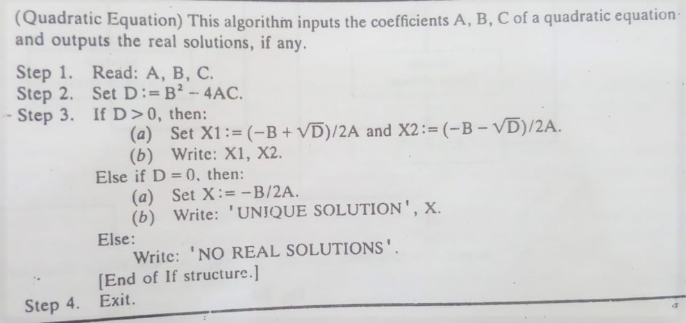
Example
The solution of quadratic equation
ax2+ bx+c=0
where a ≠ 0, have given by the quadratic formula
The quantity D=b2 – 4ac ha called the discriminant of the equation. If D is negative, then there are no real solutions. If D=0, then there is only one (double) real solution, x=-. If D is Positive, the formula gives the two distinct real solutions. The following algorithm finds the solutions of a quadratic equation.
Iteration (Repetitive flow)
One of two forms of structures with loops is the third type of logic. The following module has followed by a repeat statement for each type, termed the loop body. For clarity, the end of the structure has indicated by the declaration.
[End of loop]
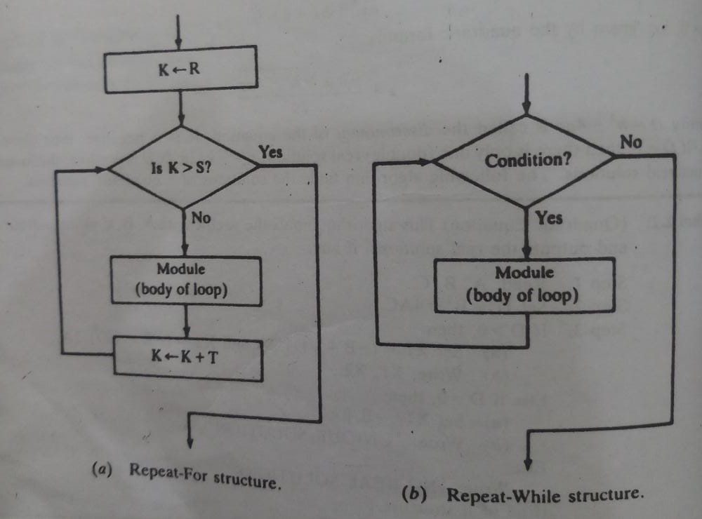
There is a distinct discussion on each form of the loop structure. The repeat-for-loop has controlled by an index variable, such as K. Normally the loop has the shape:
Here R is called the initial value, S the end value or test value, and T the increment. Observe that the body of the loop is executed first with K=R, then with K= R+T, then with K=R+2T, and so on. The cycling when K>S. The flowchart
Assumes that the increment T is positive; so that K decreases in value, then the cycling ends when K<S.
The repeat-while loop uses a condition to control the loop. The loop will usually have the form
Repeat while condition:
[Module]
[End of loop]
Note that the cycle continues until it is wrong. We highlight that the loop control condition has to be declared before the structure is first initiated and a declaration must be made on the body of the loop that alters the condition in order to finally halt the looping.
Notation: In analyzing the time and space complexity of an algorithm. We will never offer accurate numbers to set the time and space that the algorithm requires. Instead of utilizing certain common notations, also known as Asymptotic Notations. When we analyze an algorithm, we often receive a format that shows the time needed to execute the algorithm. The number of memory accesses, the number of comparisons, the time necessary for the computer to execute the algorithm code. Often this formula comprises insignificant information that does not actually tell us the time it takes.
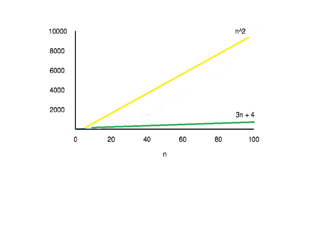
Take an example, if some algorithms have a T(n) = (n2 + 3n + 4) time complexity, which is a quadratic equation. The 3n + 4 part is negligible compared to the n2 part for the big values of n.
For n = 1000, n2 will have 1000000 while 3n + 4 will have 3004.
In addition, the consistent coefficients of higher-order terms are similarly disregarded. When compared with the execution durations of the two methods. A 200 n2 the method takes a time quicker than some other n3 time algorithm, for a value greater than 200 n. Since we are concerned solely with the asymptotic behavior of the function growth, we also may disregard the constant factor.
Asymptotic Behaviour
The phrase asymptotic implies to randomly approach a value or curve (i.e., as some sort of limit is taken). Remember that in high school you study limits, it is the same thing. The only difference here is that we do not have to find the value of any expression. Where n is near a limit or infinity. But we use the same model in the event of asymptotic notations, to ignore the constant factors. The insignificant portions of an expression and development in a single coefficient. A better way of representing the complexities of algorithms. To explain this, let’s take an example:
If we have two algorithms that show the time necessary for the execution of the following expressions:
Expression 1: (20n2 + 3n – 4)
Expression 2: (n3 + 100n – 2)
Now we need only worry about how the function will expand. When the value of n(input) increases, and that depends solely on Expression 1 n2 and Expression 2 n3. Therefore we can claim that merely analyzing the most power-coefficient and disregarding. Other constants(20 in 20n2), and inconsequential portions, for which time-run is represented by the formula 2. Will be quicker than the other approach (3n – 4 and 100n – 2).
The key concept to get things manageable is to toss aside the less important component. All we need to do is analyze the method first to get the expression. Then analyze how it grows with the growth of the input(s).
Types of Notations
In order to reflect the growth of any algorithm. We use three kinds of asymptotic. Notations as to the input increase:
The Big Theta Notation (Θ)
The Big Oh Notation (O)
Big Omega Notation (Ω)
Big Theta Notation (Θ)
When we state that the timescales indicated by the large notation are tight. We imply that the time competitiveness is like the mean value or range within. Which time the algorithm will really executed. For example, if the complexity of the time has expressed in an algorithm by equation 3n2 + 5n and we are using this Big- Tel notation, then the complexity of the time would be the same (n2), disregarding the constant-coefficient and omitting the unimportant component, which is 5n.
This indicates that the time for access to any input n is between k1 * n2 and k2 * n2, where k1, k2 have two constants, and that this means that the equation representing the development of the algorithm has tightly bound.
Big Oh Notation (O)
The top limit of the algorithm or worst case of a method has known as this notation. It informs us that for every number of n, a given function is never longer than a certain duration. Therefore, since we already have the large notation, which is a very nightmare for all algorithms, we require this representation. The question is: To explain that, let’s take a simple example. Consider the Linear Search method for an array item, searching for a specified number one by one.
In the worst scenario, we discover the element or number. We are looking for at the end, beginning on the foreside of the table. This leads to a time complexity of n, where n indicates the number of total items. However, the element that we look for is the first member in the array, thus the time complexity is 1.
In this case, now, saying that the large-to-band or close-bound time complexity for linear search is a total iv(n). Will always mean that the time needed is related to n. Since that is the correct way to represent the average time complexity. But if we use the great-to-band notation, we mean that the time complexity is O (n). This is why most of the time because it makes more sense. The Big-O notation has used to describe the time complexity of any method.
Big Omega Notation (Ω)
Big Omega notation has used to define any algorithm’s lower limit. We can tell the best case using any algorithm. This shows the least necessary time for each method, hence the best case of any algorithm, for all input values.
In simple words, if we are a time complexity in the form of a large-talk for any algorithm. We mean the algorithm takes at least that much time to perform. It can certainly take longer than that.